Models and Modelling in Science Education
In almost all the reform-based documents, models have consistently been recognized as one of the major unifying ideas that transcend disciplinary boundaries and pervade all scientific, mathematical, and technological fields (American Association for the Advancement of Science, 1989; National Research Council, 1996).
According to (Gilbert, 2000), a model is a representation of a phenomenon, an object, or an idea. In science, a model is the outcome of representing an object, phenomenon or idea (the target) with a more familiar one (the source) (Tregidgo & Ratcliffe, 2000). For example, one model of the structure of an atom (target) is the arrangement of planets orbiting the Sun (source) (Tregidgo & Ratcliffe, 2000; Ornek, 2008).
The relationship between the model and what is modeled depends on one’s
philosophical standpoint and ontological and epistemological beliefs (Lesh & Doerr, 2003).Hestenes (1987) describes a model as a representation of structure in a physical system.He also states that a model is a substitute object, a conceptual representation of a real thing.
According to (Jonassen, Strobel, & Gottdenker , 2005) a model is an artifact representative of a real object or of an internal interpretation of something real, often represented on a computer screen.
According to (Schwarz et al., 2009), a scientific model can be defined as a representation of structure that abstracts and simplifies a system to allow one to make explanations and predictions. Models may include physical objects, analogies, diagrams, graphs, computer programs, and mathematical relationships (Ling et al., 2012). Modelling has been also described as making the connection between the target and the analogue (Duit et al., 2001). When considering models, links are formed between an analogue and the source where the analogue is a symbolic representation (Chittleborough & Treagust ,2007). In Physics Education, Hestenes and his colleagues have been advocating a model-based instructional approach (or modeling instruction) for more than 20 years (Hestenes , 1987; Wells et al. ,1995). In their model-based introductory Physics curriculum on mechanics, for instance, course content is organized around a small set of basic mathematical models evolving with progressively increased empirical and rational complexity and instruction is organized into modeling cycles which move learners systematically through all phases of model development, evaluation, and application in concrete situations (Ling et al., 2012). According to Hestenes (1999), traditional physics courses lay heavy emphasis on problem solving and these results on the undesirable consequence of directing student attention to problems and their solutions as units of scientific knowledge. Modelling theory indicates us that these are the wrong units; the correct units are the models. Problem solving is important, but it should be subservient to modelling. Hestenes (1999) states that most physics and generally science/engineering problems are solved by constructing or selecting a model, from which the answer to the problem is extracted by model-based inference. In a profound sense the model provides the solution to the problem. Thus, an emphasis on models and modelling simplifies the problem and organizes a physics course into understandable units.
According to Hestenes (1999), model specification is composed by a model which describes (or specifies) four types of structure, each with internal and external components, considered as modelling indicators:
· systemic structure which specifies composition (internal parts of the system), environment (external agents linked to the system), connections (external and internal causal links)
· geometric structure which specifies position with respect to a reference frame (external geometry), configuration (geometric relations among the parts)
· temporal structure which specifies change in state variables (system properties), change by explicit functions of time and change by differential equations with interaction laws
· interaction structure which specifies interaction laws expressing interactions among causal links, usually as function of state variables
According to (Xie, et.al., 2011) we should differentiate the terms “modeling” and “simulation”. When studying the function or behavior of a system that involves time varying properties, we should use the term “simulations” and if only the structure or configuration of a system is concerned, we should use the term “models”.
According to (Jonassen et al., 2005) simulation is an executable model in connection with computer-software that allows a learner to manipulate variables and processes and observe results. Alessi and Trollip (2001) define simulations as a representation of ‘some phenomenon or activity that users learn about through interaction with the simulation’. In this definition, the term ‘interaction’ implies that the learner and the simulation communicate interactively in some way.
Stratford (1997) reviewed the research on computer simulations and models in precollege classrooms and differentiated between a model and a simulation by defining a model as "a scientific construct designed to imitate a real-world phenomenon" and a simulation as "a computer program based on a model".
In literature another term used is that of the ‘dynamic modeling”, which resembles to simulation.
After the clarification between modelling and simulation, we consider that the term that best describes the models we use in science education is “models of simulations”.
According to Hestrenes (1987), to fully describe a model and the corresponding simulation, we need: a) descriptive variables which represent an object’s characteristics; i.e. object variables, state variables, and interaction variables and b) equations of the model which describe the model’s structure.
The variables and the equations are in full correspondence with the four types of structure of models described above (Hestenes, 1999).
For example, the equations are in alignment with the “interaction structure which specifies interaction laws expressing interactions among causal links, usually as function of state variables”.
A number of science educators suggest that “models of simulations” offer considerable potential for the enhancement of the teaching of science concepts enabling students to modify rules and variables to explore the science of a model, to question and test hypotheses (Enyedy & Goldberg, 2004). They also offer simultaneous representations of the real and theoretical behaviours of a system (McFarlane & Sakellariou, 2002) and support activities that would actively engage the learner and, finally, they offer visualization of choices and consequent effects (Rogers, 2004).
When learners build “models of simulations”, there is an interplay between their current understanding of the target and the computational models they create. During the engagement with the model, there is an interaction between learners’ growing intuition and the underlying viewpoint of the simulation (Jonassen et al., 2005).
Numerous kinds of models can be used to represent phenomena in the world or the mental representations that learners construct to represent them. Harris (1999)
described three kinds of models: theoretical models, experimental models, and data models. Giere (1999) described several kinds of models, including representational
models, abstract models (mathematical models), and theoretical models. Lehrer and Schauble (2003) described a continuum of model types, including physical models, representational systems , syntactic models, and hypothetical–deductive models (formal abstractions). de Jong and van Joolingen (1998) distinguished between conceptual and operational models, where conceptual models hold principles, concepts, and facts that make up the system being modeled, and operational models include sequences of cognitive and no cognitive operations (e.g., procedures). Ornek (2005) described kinds of models: mental models, conceptual models, mathematical models, computer models and physics models.
In all these models we should consider what are the main design concepts and principles in a computational environment that it should support learners in engagement in scientific activities and acquisition of scientific abilities.
The Computational Experiment
According to (Landau et al., 2008) the ensuing decade has strengthened the view that the physics community is well served by having Computational Physics(CP) as a prominent member of the broader computational science and engineering (CSE) community.
Computational Science (the term is used identically to computational science and engineering) is the use of mathematics and computers to explore “real world” problems in science and is a multidisciplinary activity which brings together people from a variety of disciplines.
According to (Vojta, 2006) Computational Physics ( CP) is the 3rd independent scientific methodology that has arisen over the last 20 years or so, it shares characteristics with both theory and experiment, and it requires interdisciplinary skills in science, mathematics, computer science. He also clearly states that Computational Science is different from Computer Science.
Landau and Yasar (2003), state that Computational Science (CS) sometimes denotes the multidisciplinary combination of computational techniques, tools, and knowledge needed to solve modern scientific and engineering problems. At other times it denotes
science or engineering that uses computer simulations as its basis, and sometimes it
denotes the research and development of computational skills and tools needed for
applications.
The original view of CS, shown on the left side of Figure 1, was the intersection
of applied mathematics, computer science, and application sciences. This early view is now being replaced by the one represented by the right side of Figure 1.
Figure 1. The knowledge area of Computational Science
The core of CS may be thought of as its collection of computational tools and methods and its problem-solving mindset, which uses knowledge in one discipline to solve problems in another. This CS core is now being incorporated into computational science courses and books that combine scientific problem solving with computation and into curricula at various levels of education.
Computational Physics helps learners to solve a physics problem using computer simulations and this includes diverse tasks, like:
· formulating the physics problem in a way suitable for simulations
· choosing an efficient computational algorithm
· writing and testing computer code
· running the simulations and collecting numerical data
· analyzing and visualizing the data obtained
· extracting the solution of the physics problem
According to the scientific community, there is clear need for Computational Physics courses that:
· focus on the science aspects of computational physics
· give students hands-on experience in designing and running computer simulations
· play a role similar to that of laboratory courses for experiment
One of the crucial components of CP is the abstraction of a physical phenomenon to a conceptual model and its translation into a computational model that can be validated. This leads us to the notion of a computational experiment where the model and the computer take the place of the ‘classical’ experimental set-up, and simulation replaces the experiment as such. Sloot (1994) identifies three major phases in the process of the development of a computer experiment: a. The modelling phase: the first step to simulation is the development of an abstract model of the physical system under study, b. The simulation phase: this refers to methods that make the underlying physical models discrete in time or stochastic using methods from numerical analysis and c. The computational phase: in this phase we concentrate on the mapping of the simulation techniques to source code including algorithms and the implementation using software or a programming language.
Landau et al. (2008) suggests an approach similar to Sloot’s approach, which takes the form: Problem (from science), b. Modelling (mathematical relations between selected entities and variables), c. Simulation Method (time driven, event driven, stochastic), d. Development of algorithm, e. Implementation of the algorithm (using Java, Mathematica, Fortran etc) and f. Assessment , Visualization and Exploration of the results and comparison with real data
According to Landau et al. (2008), Computational Physics (CP) and Computational Experiment (CE) provide a broader, more balanced, and more flexible education than a traditional physics major. Moreover, presenting physics within a scientific problem solving paradigm is a more effective and efficient way to teach physics than the traditional approach. In this framework, being able to transform a theory into an algorithm requires significant theoretical insight, detailed physical and mathematical understanding and a mastery of the art of programming and the actual debugging and testing. The organization of scientific programs is analogous to experimentation, with the numerical simulations of nature being essentially virtual experiments.
Tobochnik and Gould (2008) argue that CP should be incorporated into the curriculum because it can elucidate the physics. Computation is both a language and a tool and, in analogy to models expressed in mathematical statements, CP models are expressed as algorithms which in many cases are explicit implementations of mathematics. An advantage of the computational approach is that it is necessary to be explicit about which symbols represent variables and which represent initial conditions and parameters, boundary conditions, restrictions of the solutions etc.
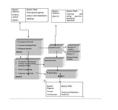
Shunn and Klahr (1995) in order to describe inquiry based learning as a search process introduced the hypothesis space and the experimental space. In their model the hypothesis space contains all rules and variables describing the specific domain, while the experimental space consists of all experiments that can be implemented within this domain. Psycharis (2011; 2013) extended these spaces in order to include the computational experiment approach and suggested three spaces for the computational experiment, namely:
1. The hypotheses space, where the learners, in cooperation with the Instructor, decide, clarify and state the hypotheses of the problem to be studied, as well as the variables and concepts to be used and the relations between them..
2. The experimental space, where the computational experiment actually takes place and implements the “model of simulation”, replacing the classical experimental and learners are engaged in the scientific method.
3. The prediction space, where the results, conclusions or solutions formulated in the experimental space, are checked with the analytical (mathematical) solution as well as with data from the real world and help learners towards predictions for other phenomena.
In almost all the reform-based documents, models have consistently been recognized as one of the major unifying ideas that transcend disciplinary boundaries and pervade all scientific, mathematical, and technological fields (American Association for the Advancement of Science, 1989; National Research Council, 1996).
According to (Gilbert, 2000), a model is a representation of a phenomenon, an object, or an idea. In science, a model is the outcome of representing an object, phenomenon or idea (the target) with a more familiar one (the source) (Tregidgo & Ratcliffe, 2000). For example, one model of the structure of an atom (target) is the arrangement of planets orbiting the Sun (source) (Tregidgo & Ratcliffe, 2000; Ornek, 2008).
The relationship between the model and what is modeled depends on one’s
philosophical standpoint and ontological and epistemological beliefs (Lesh & Doerr, 2003).Hestenes (1987) describes a model as a representation of structure in a physical system.He also states that a model is a substitute object, a conceptual representation of a real thing.
According to (Jonassen, Strobel, & Gottdenker , 2005) a model is an artifact representative of a real object or of an internal interpretation of something real, often represented on a computer screen.
According to (Schwarz et al., 2009), a scientific model can be defined as a representation of structure that abstracts and simplifies a system to allow one to make explanations and predictions. Models may include physical objects, analogies, diagrams, graphs, computer programs, and mathematical relationships (Ling et al., 2012). Modelling has been also described as making the connection between the target and the analogue (Duit et al., 2001). When considering models, links are formed between an analogue and the source where the analogue is a symbolic representation (Chittleborough & Treagust ,2007). In Physics Education, Hestenes and his colleagues have been advocating a model-based instructional approach (or modeling instruction) for more than 20 years (Hestenes , 1987; Wells et al. ,1995). In their model-based introductory Physics curriculum on mechanics, for instance, course content is organized around a small set of basic mathematical models evolving with progressively increased empirical and rational complexity and instruction is organized into modeling cycles which move learners systematically through all phases of model development, evaluation, and application in concrete situations (Ling et al., 2012). According to Hestenes (1999), traditional physics courses lay heavy emphasis on problem solving and these results on the undesirable consequence of directing student attention to problems and their solutions as units of scientific knowledge. Modelling theory indicates us that these are the wrong units; the correct units are the models. Problem solving is important, but it should be subservient to modelling. Hestenes (1999) states that most physics and generally science/engineering problems are solved by constructing or selecting a model, from which the answer to the problem is extracted by model-based inference. In a profound sense the model provides the solution to the problem. Thus, an emphasis on models and modelling simplifies the problem and organizes a physics course into understandable units.
According to Hestenes (1999), model specification is composed by a model which describes (or specifies) four types of structure, each with internal and external components, considered as modelling indicators:
· systemic structure which specifies composition (internal parts of the system), environment (external agents linked to the system), connections (external and internal causal links)
· geometric structure which specifies position with respect to a reference frame (external geometry), configuration (geometric relations among the parts)
· temporal structure which specifies change in state variables (system properties), change by explicit functions of time and change by differential equations with interaction laws
· interaction structure which specifies interaction laws expressing interactions among causal links, usually as function of state variables
According to (Xie, et.al., 2011) we should differentiate the terms “modeling” and “simulation”. When studying the function or behavior of a system that involves time varying properties, we should use the term “simulations” and if only the structure or configuration of a system is concerned, we should use the term “models”.
According to (Jonassen et al., 2005) simulation is an executable model in connection with computer-software that allows a learner to manipulate variables and processes and observe results. Alessi and Trollip (2001) define simulations as a representation of ‘some phenomenon or activity that users learn about through interaction with the simulation’. In this definition, the term ‘interaction’ implies that the learner and the simulation communicate interactively in some way.
Stratford (1997) reviewed the research on computer simulations and models in precollege classrooms and differentiated between a model and a simulation by defining a model as "a scientific construct designed to imitate a real-world phenomenon" and a simulation as "a computer program based on a model".
In literature another term used is that of the ‘dynamic modeling”, which resembles to simulation.
After the clarification between modelling and simulation, we consider that the term that best describes the models we use in science education is “models of simulations”.
According to Hestrenes (1987), to fully describe a model and the corresponding simulation, we need: a) descriptive variables which represent an object’s characteristics; i.e. object variables, state variables, and interaction variables and b) equations of the model which describe the model’s structure.
The variables and the equations are in full correspondence with the four types of structure of models described above (Hestenes, 1999).
For example, the equations are in alignment with the “interaction structure which specifies interaction laws expressing interactions among causal links, usually as function of state variables”.
A number of science educators suggest that “models of simulations” offer considerable potential for the enhancement of the teaching of science concepts enabling students to modify rules and variables to explore the science of a model, to question and test hypotheses (Enyedy & Goldberg, 2004). They also offer simultaneous representations of the real and theoretical behaviours of a system (McFarlane & Sakellariou, 2002) and support activities that would actively engage the learner and, finally, they offer visualization of choices and consequent effects (Rogers, 2004).
When learners build “models of simulations”, there is an interplay between their current understanding of the target and the computational models they create. During the engagement with the model, there is an interaction between learners’ growing intuition and the underlying viewpoint of the simulation (Jonassen et al., 2005).
Numerous kinds of models can be used to represent phenomena in the world or the mental representations that learners construct to represent them. Harris (1999)
described three kinds of models: theoretical models, experimental models, and data models. Giere (1999) described several kinds of models, including representational
models, abstract models (mathematical models), and theoretical models. Lehrer and Schauble (2003) described a continuum of model types, including physical models, representational systems , syntactic models, and hypothetical–deductive models (formal abstractions). de Jong and van Joolingen (1998) distinguished between conceptual and operational models, where conceptual models hold principles, concepts, and facts that make up the system being modeled, and operational models include sequences of cognitive and no cognitive operations (e.g., procedures). Ornek (2005) described kinds of models: mental models, conceptual models, mathematical models, computer models and physics models.
In all these models we should consider what are the main design concepts and principles in a computational environment that it should support learners in engagement in scientific activities and acquisition of scientific abilities.
The Computational Experiment
According to (Landau et al., 2008) the ensuing decade has strengthened the view that the physics community is well served by having Computational Physics(CP) as a prominent member of the broader computational science and engineering (CSE) community.
Computational Science (the term is used identically to computational science and engineering) is the use of mathematics and computers to explore “real world” problems in science and is a multidisciplinary activity which brings together people from a variety of disciplines.
According to (Vojta, 2006) Computational Physics ( CP) is the 3rd independent scientific methodology that has arisen over the last 20 years or so, it shares characteristics with both theory and experiment, and it requires interdisciplinary skills in science, mathematics, computer science. He also clearly states that Computational Science is different from Computer Science.
Landau and Yasar (2003), state that Computational Science (CS) sometimes denotes the multidisciplinary combination of computational techniques, tools, and knowledge needed to solve modern scientific and engineering problems. At other times it denotes
science or engineering that uses computer simulations as its basis, and sometimes it
denotes the research and development of computational skills and tools needed for
applications.
The original view of CS, shown on the left side of Figure 1, was the intersection
of applied mathematics, computer science, and application sciences. This early view is now being replaced by the one represented by the right side of Figure 1.
Figure 1. The knowledge area of Computational Science
The core of CS may be thought of as its collection of computational tools and methods and its problem-solving mindset, which uses knowledge in one discipline to solve problems in another. This CS core is now being incorporated into computational science courses and books that combine scientific problem solving with computation and into curricula at various levels of education.
Computational Physics helps learners to solve a physics problem using computer simulations and this includes diverse tasks, like:
· formulating the physics problem in a way suitable for simulations
· choosing an efficient computational algorithm
· writing and testing computer code
· running the simulations and collecting numerical data
· analyzing and visualizing the data obtained
· extracting the solution of the physics problem
According to the scientific community, there is clear need for Computational Physics courses that:
· focus on the science aspects of computational physics
· give students hands-on experience in designing and running computer simulations
· play a role similar to that of laboratory courses for experiment
One of the crucial components of CP is the abstraction of a physical phenomenon to a conceptual model and its translation into a computational model that can be validated. This leads us to the notion of a computational experiment where the model and the computer take the place of the ‘classical’ experimental set-up, and simulation replaces the experiment as such. Sloot (1994) identifies three major phases in the process of the development of a computer experiment: a. The modelling phase: the first step to simulation is the development of an abstract model of the physical system under study, b. The simulation phase: this refers to methods that make the underlying physical models discrete in time or stochastic using methods from numerical analysis and c. The computational phase: in this phase we concentrate on the mapping of the simulation techniques to source code including algorithms and the implementation using software or a programming language.
Landau et al. (2008) suggests an approach similar to Sloot’s approach, which takes the form: Problem (from science), b. Modelling (mathematical relations between selected entities and variables), c. Simulation Method (time driven, event driven, stochastic), d. Development of algorithm, e. Implementation of the algorithm (using Java, Mathematica, Fortran etc) and f. Assessment , Visualization and Exploration of the results and comparison with real data
According to Landau et al. (2008), Computational Physics (CP) and Computational Experiment (CE) provide a broader, more balanced, and more flexible education than a traditional physics major. Moreover, presenting physics within a scientific problem solving paradigm is a more effective and efficient way to teach physics than the traditional approach. In this framework, being able to transform a theory into an algorithm requires significant theoretical insight, detailed physical and mathematical understanding and a mastery of the art of programming and the actual debugging and testing. The organization of scientific programs is analogous to experimentation, with the numerical simulations of nature being essentially virtual experiments.
Tobochnik and Gould (2008) argue that CP should be incorporated into the curriculum because it can elucidate the physics. Computation is both a language and a tool and, in analogy to models expressed in mathematical statements, CP models are expressed as algorithms which in many cases are explicit implementations of mathematics. An advantage of the computational approach is that it is necessary to be explicit about which symbols represent variables and which represent initial conditions and parameters, boundary conditions, restrictions of the solutions etc.
Shunn and Klahr (1995) in order to describe inquiry based learning as a search process introduced the hypothesis space and the experimental space. In their model the hypothesis space contains all rules and variables describing the specific domain, while the experimental space consists of all experiments that can be implemented within this domain. Psycharis (2011; 2013) extended these spaces in order to include the computational experiment approach and suggested three spaces for the computational experiment, namely:
1. The hypotheses space, where the learners, in cooperation with the Instructor, decide, clarify and state the hypotheses of the problem to be studied, as well as the variables and concepts to be used and the relations between them..
2. The experimental space, where the computational experiment actually takes place and implements the “model of simulation”, replacing the classical experimental and learners are engaged in the scientific method.
3. The prediction space, where the results, conclusions or solutions formulated in the experimental space, are checked with the analytical (mathematical) solution as well as with data from the real world and help learners towards predictions for other phenomena.